5 Easy Steps for Interpreting Linear Regression F Statistic
Interpretation of Linear Regression
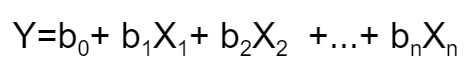
Linear Regression is the most talked-about term for those who are working on ML and statistical analysis. Linear Regression, as the name suggests, simply means fitting a line to the data that establishes a relationship between a target 'y' variable with the explanatory 'x' variables. It can be characterized by the equation below:
Let us take a sample data set which I got from a course on Coursera named "Linear Regression for Business Statistics" .
The data set looks like :
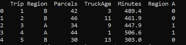
The interpretation of the first row is that the first trip took a total of 489.4 minutes to deliver 42 parcels driving through a truck which was 3 years old to a Region B. Here, the time taken is our target variable and 'Region A', 'TruckAge' and 'Parcels' are our explanatory variables. Since, the column 'Region' is a categorical variable, it should be encoded with a numeric value.
If we have 'n' numbers of labels in our categorical variable then 'n-1' extra columns are added to uniquely represent or encode the categorical variable. Here, 1 in RegionA indicates that the trip was to region A and 0 indicates that the trip was to region B.
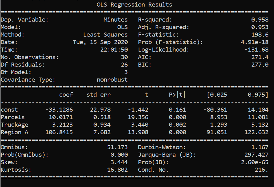
Above is the summary of linear regression performed in the data set. Therefore, from the results above, our linear equation would be :
Minutes= -33.1286+10.0171*Parcels + 3.21* TruckAge + 106.84* Region A
Interpretation:
b₁=10.0171: It means that it will take 10.0171 extra minutes to deliver if the number of parcels increases by 1, other variables remaining constant.
b₂=3.21: It means that it will take 3.21 more minutes to deliver if the truck age increases by 1 unit , other variables remaining constant.
b₃=106.84: It means that it will take 106.84 more minutes when the delivery is done to Region A as compared with Region B, other variables remaining constant. There's always a reference variable to compare with when it comes to interpretation of coefficient of a categorical variable and here, the reference is to Region B as we have assigned 0 to region B.
b₀=-33.1286 : It mathematically means the amount of time taken to deliver 0 parcels by a truck of age 0 to region B. This doesn't make any sense from a business perspective. Sometimes the intercept may have some meaningful insights to give and sometimes it is just there to fit the data.
But, we have to check if this is what defines the relationship between our x variables and y variable. The fit we obtained is an estimate only on a sample data and it is not yet acceptable to conclude that this same relationship may exist on the real data. We must check if the parameters we got are statistically significant or are just there to fit the data to the model. Therefore, it is extremely crucial that we examine the goodness of fit and the significance of the x variables.
Hypothesis Testing
Hypothesis testing can be done by various ways like the t-statistics test, confidence interval test and the p-value test. Here, we're going to examine the p values corresponding to each of the coefficients.
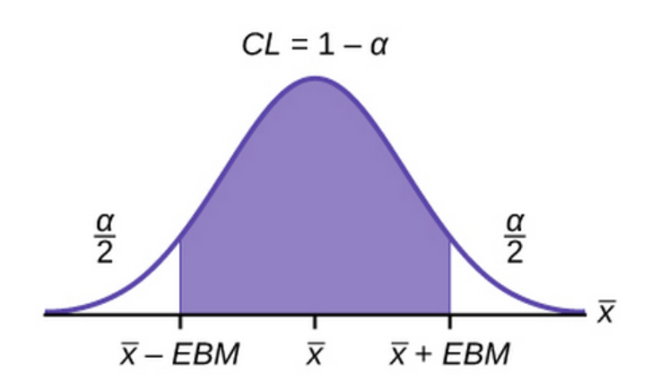
For every hypothesis testing, we define a confidence interval i.e (1-alpha), such that this region is called the accepting region and the remaining regions with area alpha/2 on both sides ( in a two tailed test) are the rejection region. In order to do a hypothesis test we must assume a null hypothesis and an alternate hypothesis.
Null Hypothesis : This X variable has no effect on the Y variable i.e H₀: b=0
Alternate Hypothesis: This X variable has effect on the Y variable i.e
H₁: b ≠0
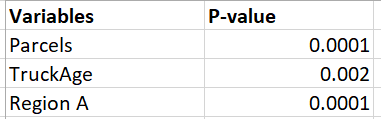
Null hypothesis is only accepted if the p-value is greater than the value of alpha/2. As we can see from the table above, all the p values are less than 0.05/2 ( if we take a 95% confidence interval). This means the p value lies somewhere in the rejecting region and therefore, we can reject the null hypothesis. Thus, all of our x variables are important in defining the y variable. And, the coefficient of the x variables are statistically significant and are not there just to fit the data to the model.
Our Own hypothesis testing
The above hypothesis was the default hypothesis done by the statsmodel itself. Lets us assume that we have a popular belief that the amount of time taken to make the delivery increases by 5 minutes with unit increase in the truck age , keeping all other variables constant. Now we can test if this belief still holds in our model.
Null hypothesis H₀ : b₂=5
Alternate Hypothesis H₁ : b₂ ≠5
The OLS Regression results show that the range of values of the coefficient of TruckAge is : [1.293 , 5.132] . For these values of coefficient, the variable is considered to be statistically significant. The midpoint of the interval [1.293 , 5.132] is our estimated coefficient given by the model. Since our test statistic is 5 minutes and it lies within the range [1.293 , 5.132], we cannot ignore the null hypothesis. Therefore, we cannot ignore the popular belief that it takes extra 5 minutes to deliver through a unit year older truck. In the end, b₂ is taken 3.2123 , its just that the hypothesis is providing enough evidence that the b₂ that we have estimated is a good estimation. However, 5 minutes can also be a possible good estimation of b₂.
Measuring the goodness of fit
The R square value is used as a measure of goodness of fit. The value 0.958 indicates that 95.8% of variations in Y variable can be explained by our X variables. The remaining variations in Y go unexplained.
Total SS= Regression SS + Residual SS
R square= Regression SS/ Total SS
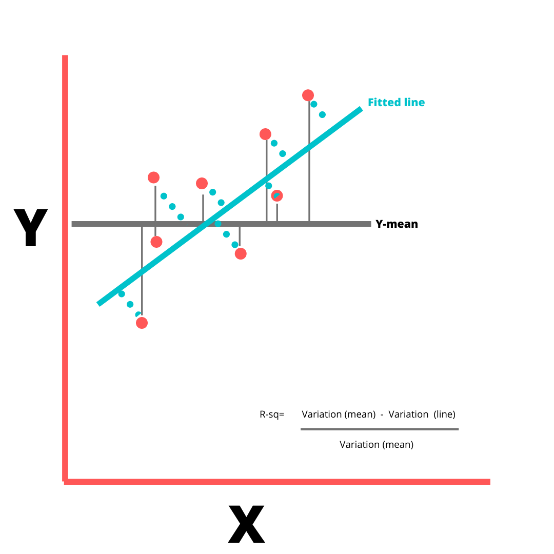
Lowest value of R square can be 0 and highest can be 1. A low R-squared value indicates a poor fit and signifies that you might be missing some important explanatory variables. The value of R- square increases by increase in X variables, irrespective of whether the added X variable is important or not. So to adjust with this, there's Adjusted R square value that increases only if the additional X variable improves the model more than would be expected by chance and decreases when additional variable improves the model by less than expected by chance.
Residual Plots
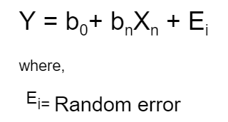
There are some assumptions made about this random error before the linear regression is performed.
- The mean of the random error is 0 .
- The random errors have a constant variance.
- The errors are normally distributed.
- The error instances are independent of each other
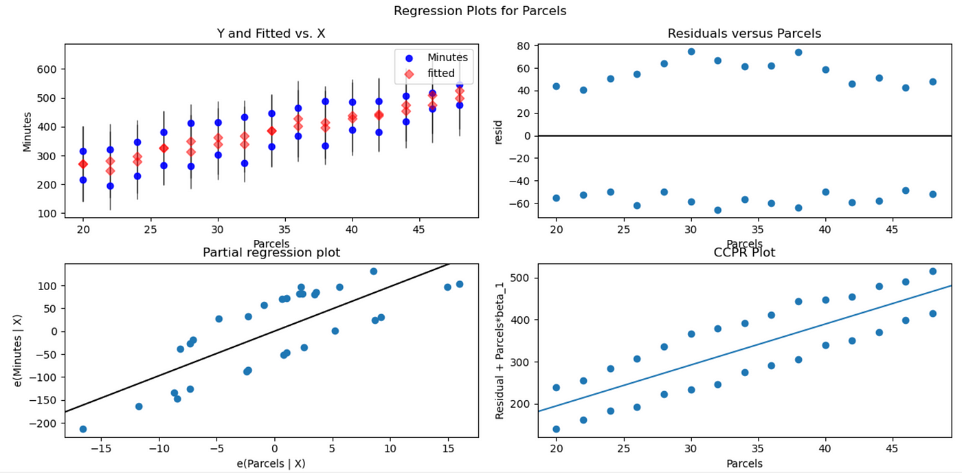
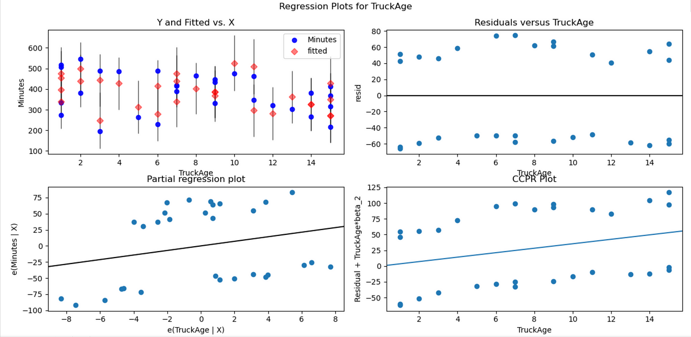
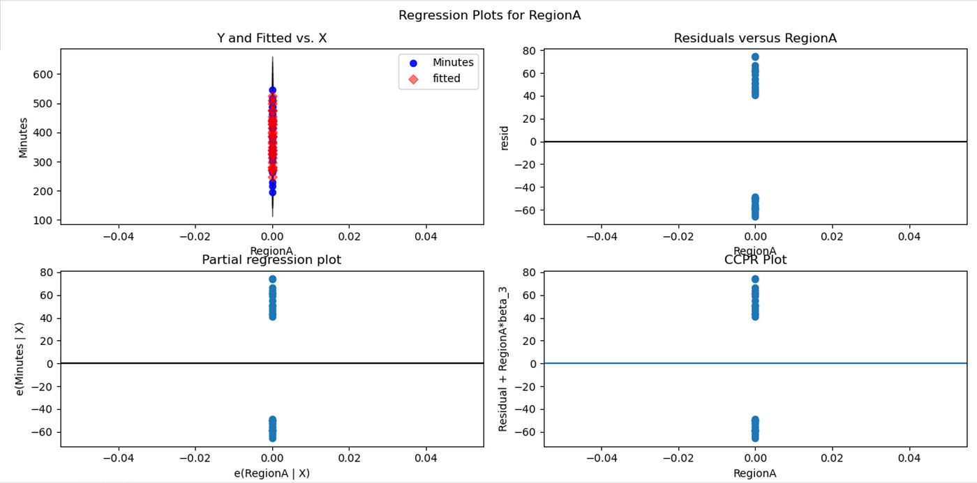
In the plots above, the residuals vs X variable plots show if our model assumptions are violated or not. In fig-6 , the residual vs parcels plot seems to be scattered. The residuals are distributed randomly around zero and seem to have a constant variance. Same is the case with residual plots of the other x variables. Therefore, the initial assumptions about the random error still hold. If there were any curvature/trends among the residuals or the variance seems to be changing with the x variable (or any other dimension) then, it could signify that there's a huge problem with our linear model as the initial assumptions violated. In such cases, box cox method should be performed. It is a process where the problematic x variable is subjected to transformations like log or square root so that the residue would have a constant variance. The kind of transformation to do with the x variable is like a hit and trial method.
Multi-collinearity
Multi-collinearity occurs when there are high correlations among independent variables in a multiple regression model that can causes insignificant p values although the independent variables are tested important individually.
Let us consider the data set :
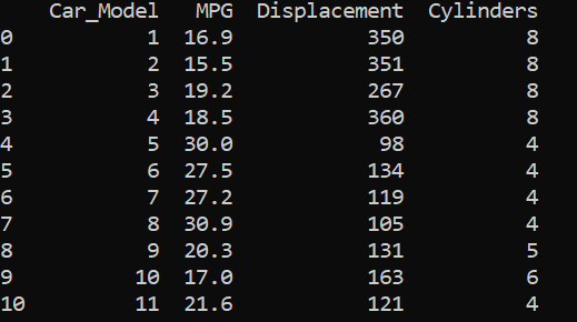
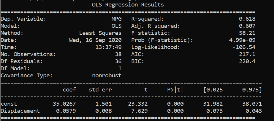
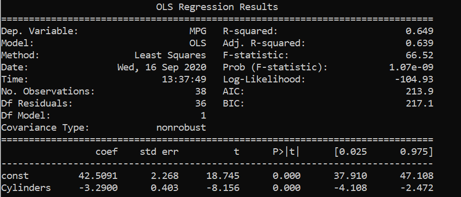
From the above results, we saw that displacements and cylinders seem to be statistically important variables as their p-values are less than alpha/2 in the first two results where single variable linear regression was performed.
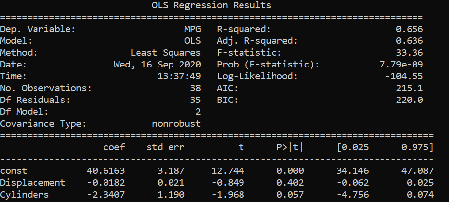
When multi linear regression was performed, both the x variables turned out to be unimportant as their p-values are greater than alpha/2 . However, both the variables are important as per the previous two simple regressions. This might be caused by multicollinearity in the data set.
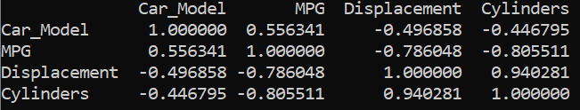
We can see that the displacement and cylinders are strongly correlated with each other with a correlation coefficient of 0.94. Therefore, to deal with such issues, one of the highly correlated variables should be avoided in linear regression.
The overall code can be found here.
Thanks for reading!
Source: https://towardsdatascience.com/interpretation-of-linear-regression-dba45306e525
Postar um comentário for "5 Easy Steps for Interpreting Linear Regression F Statistic"